Population Stability Index
The population stability index (PSI) summarises in one number how much a distribution has shifted between two samples, for example between training data and what the model sees in production. It bins both distributions and compares the share of items in each bin.
It is one of the ways of detecting drift.
Example
A random forest predicts (log) bulldozer prices from the Blue Book for Bulldozers dataset. It trains on sales before October 2011 and validates on sales after, scoring 0.988 on training and 0.894 on validation. Has the population shifted between the two?
Calculating PSI
- Take a reference distribution and a target distribution.
- Choose
n_binsbins from the reference distribution, either:fixed: equal-width bins between its minimum and maximum, orquantile: bins holding an equal number of reference items.
- Compute the proportion of items in each bin, for both distributions.
- Replace any zero proportions with a small
epsilon, so the formula never divides by zero or takes the log of zero. - Sum over the bins:
where and are the reference and target proportions in bin . Every term is non-negative, and swapping reference and target gives the same answer.
def get_population_proportions(ref, target, n_bins: int, bin_mode: str, eps: float = 0.001):
    if bin_mode == "fixed":
        ref_counts, breakpoints = np.histogram(ref, n_bins)
    elif bin_mode == "quantile":
        breakpoints = np.quantile(ref, np.linspace(0, 1, n_bins + 1))
        ref_counts = np.histogram(ref, breakpoints)[0]
    target_counts = np.histogram(target, breakpoints)[0]
    ref_props = ref_counts / ref_counts.sum()
    target_props = target_counts / target_counts.sum()
    return np.where(ref_props == 0, eps, ref_props), np.where(target_props == 0, eps, target_props)


def psi(ref, target, n_bins: int, bin_mode: str, eps: float = 0.001) -> float:
    r, t = get_population_proportions(ref, target, n_bins, bin_mode, eps)
    return np.sum((t - r) * np.log(t / r))
One trap: np.histogram silently drops values outside the outer bin edges. If the target has values beyond the reference's range, which is exactly the kind of shift we're looking for, they vanish from the count. Setting the first and last breakpoints to -np.inf and np.inf fixes it.
On the predictions, PSI is 0.053 with fixed bins and 0.056 with quantile bins.
The usual rule of thumb:
| PSI | Interpretation |
|---|---|
| below 0.1 | no significant change |
| 0.1 to 0.2 | moderate change |
| 0.2 or more | significant change |
So the model's predictions look stable between the two periods.
Visualising it
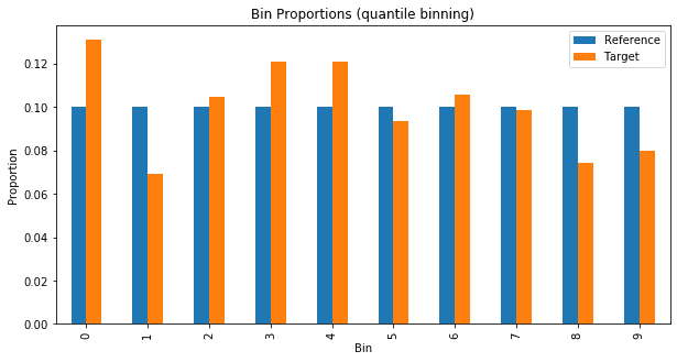
Plotting the bin proportions side by side shows where the distributions differ (quantile bins, with the validation set as the reference):
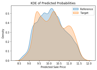
A kernel density estimate shows the same without binning, though, as the Seaborn docs warn, it can distort distributions that are bounded or not smooth:
Characteristic stability index
The same calculation applied to a single input feature, instead of the model's output, is usually called the characteristic stability index (CSI). There is no normalisation: a feature's CSI is just its PSI. Ranking features by CSI shows which inputs have shifted most:
csi = {col: psi(train_xs[col].values, valid_xs[col].values, 10, "quantile") for col in train_xs.columns}| Feature | CSI |
|---|---|
| saleElapsed | 6.16 |
| SalesID | 5.59 |
| datasource | 5.39 |
| saleYear | 5.10 |
| saleMonth | 4.98 |
Some of these are obvious given a split by date: anything derived from the sale date is bound to shift. Others, like datasource, deserve a closer look, and plotting each feature's KDE for the two periods helps.
Sources
- Checking model stability and population shift with PSI and CSI, Vinícius Trevisan
- Population Stability Index, Matthew Burke
- Measuring Data Drift: Population Stability Index, Murtuza Shergadwala
- The bulldozer model follows the fast.ai book.
Linked from
Revision log
- Migrated from data-science-notes; renamed FSI to CSI and corrected its definition
Tags: Machine Learning