Classification Metrics
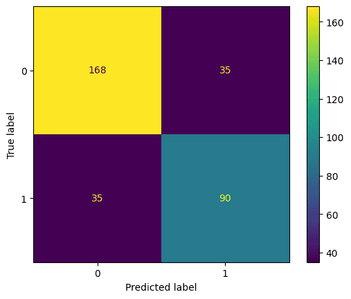
The running example is a random forest predicting survival on the Titanic, scored on a held-out test set. test_preds holds its predicted probabilities of survival.
Accuracy
Accuracy needs a threshold above which a predicted probability counts as a positive. Different thresholds give different accuracies, and the one that maximises accuracy is not necessarily the one you want:
accuracy_score(y_test, test_preds > 0.1)  # 0.607
accuracy_score(y_test, test_preds > 0.5)  # 0.787
accuracy_score(y_test, test_preds > 0.9)  # 0.753
Recall
Recall is the fraction of the actual positives that the model identified:
Lowering the threshold catches more of them: recall is 0.93 at 0.1, 0.72 at 0.5 and 0.38 at 0.9.
Precision
Precision, also called positive predictive value, is the fraction of positive predictions that were right:
It moves the other way: 0.49 at 0.1, 0.72 at 0.5, 0.94 at 0.9.
F1 score
The F1 score is the harmonic mean of precision and recall, so it weights them equally. It is 1 for perfect precision and recall and 0 if either is zero. For multi-class or imbalanced problems, average="macro" averages the per-class scores equally, "weighted" weights them by class size, and "micro" pools all predictions (for single-label problems that equals accuracy).
Confusion matrix
ROC curve
Varying the threshold trades the true positive rate (recall) against the false positive rate. The receiver operating characteristic (ROC) curve plots one against the other across all thresholds. The name comes from radar engineering in the Second World War, where it described how well receivers picked out aircraft from noise.
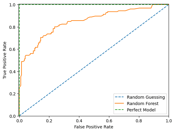
With random guessing, every gain in true positive rate costs an equal rise in false positive rate: the diagonal. A perfect model goes straight to a 100% true positive rate at a 0% false positive rate. Ours gains true positives faster than false positives up to a point, after which the false positives come faster.
We'd usually pick a threshold near the top-left corner, unless errors have unequal costs. If a false positive is more expensive than a false negative, we'd accept a lower true positive rate for a lower false positive rate. Profit Curves makes that trade-off explicit.
ROC AUC
To compare models rather than thresholds, we can measure the area under the ROC curve. 0.5 is random guessing and 1.0 is perfect; this model scores 0.847.
AUC has a second interpretation: it is the probability that a randomly chosen positive row gets a higher predicted probability than a randomly chosen negative one (ties count half). Formally, over all pairs of rows,
where is the predicted probability and the true label of row .
A consequence is that the AUC of a set can be larger than the AUC of every one of its subsets. Take two small datasets, each with one correctly and one incorrectly ordered (positive, negative) pair, so each has an AUC of 0.5:
| pred | y | pred | y | |
|---|---|---|---|---|
| 0.09 | 0 | 0.095 | 0 | |
| 0.5 | 1 | 0.41 | 1 | |
| 0.7 | 0 | 0.42 | 0 |
Combined, there are two positives and four negatives, so eight pairs. The positive at 0.41 beats two negatives and the positive at 0.5 beats three, so the AUC is . Pairs that were never compared within either subset are now compared, and they happen to be ordered correctly.
Gini and the CAP curve
The cumulative accuracy profile (CAP) sorts rows by predicted probability, highest first, and plots the cumulative number of positives captured against the number of rows taken. A random model is a straight diagonal; a perfect model captures every positive first and then flattens.
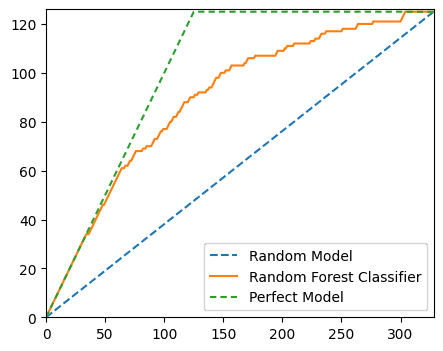
The accuracy ratio compares the area between our model's curve and the random diagonal with the same area for the perfect model:
Here that is . The accuracy ratio equals the Gini coefficient, and both equal . (On normalised axes, with the share of positives, the perfect model's area above the diagonal is , not ½, so the identity needs a little more work than it seems; this derivation goes through it.)
2 * roc_auc_score(y_test, test_preds) - 1 # 0.694The small gap between 0.697 and 0.694 comes from ties. A random forest gives many rows exactly the same probability, and sorting the CAP data by (prediction, label) in descending order puts tied positives ahead of tied negatives, which flatters the curve. roc_auc_score counts ties as half.
Precision-recall curve
The precision-recall curve plots precision against recall across thresholds. Raising the threshold usually raises precision, because the model only says "positive" when it is confident, and lowers recall, because fewer true positives clear the bar. (Precision is not guaranteed to rise at every step.) High scores on both mean the model returns mostly correct positives and most of the positives there are, so we want the curve towards the top right.
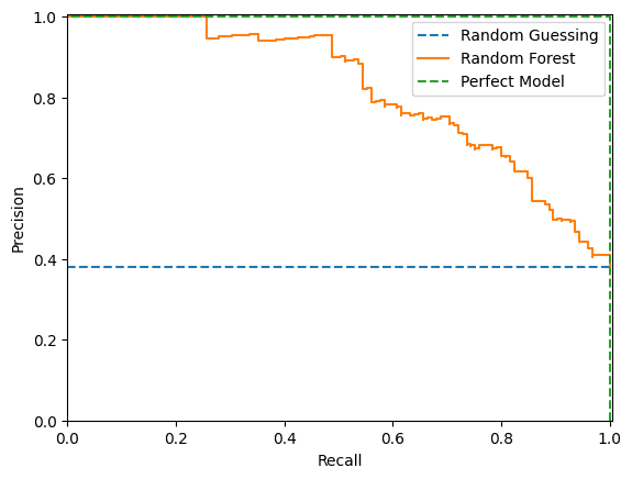
A random model gives a horizontal line at the share of positives. That makes PR curves more informative than ROC curves on imbalanced data: a model can't look good just by predicting the majority class (Saito and Rehmsmeier, 2015).
The usual summary is average precision: a step-wise sum of precision at each threshold, weighted by the increase in recall. It is not the trapezium rule; scikit-learn deliberately avoids interpolating between points, which can be over-optimistic.
-np.sum(np.diff(recall) * np.array(precision)[:-1])  # 0.820
average_precision_score(y_test, test_preds)          # 0.820
For curves that rank rows by predicted probability, see also Gain, Lift and Deciles.
Sources
- Can the ROC AUC of a total test set be larger than the AUC for any subset?
- CAP analysis
- Gini, cumulative accuracy profile and AUC
Linked from
Revision log
- Migrated from data-science-notes; corrected the Gini derivation and the description of average precision
Tags: Machine Learning