Gradient Descent

Fitting a model usually means solving an optimisation problem: find the parameters that minimise the error of the predictions, or maximise the likelihood of the data.

The gradient of a function is the vector of its partial derivatives. It points in the direction in which the function increases fastest. So to minimise a function we can pick a starting point, compute the gradient, take a small step in the opposite direction, and repeat. (To maximise, step along the gradient instead: gradient ascent, as in Logistic Regression.)

def f(x: float, y: float) -> float:
    return x**2 + y**2
 
 
def gradient_descent(learning_rate: float, iterations: int, initial_point: tuple[float, float]) -> np.ndarray:
    x, y = initial_point
    history = [(x, y)]
    for _ in range(iterations):
        x -= learning_rate * 2 * x  # ∂f/∂x = 2x
        y -= learning_rate * 2 * y  # ∂f/∂y = 2y
        history.append((x, y))
    return np.array(history)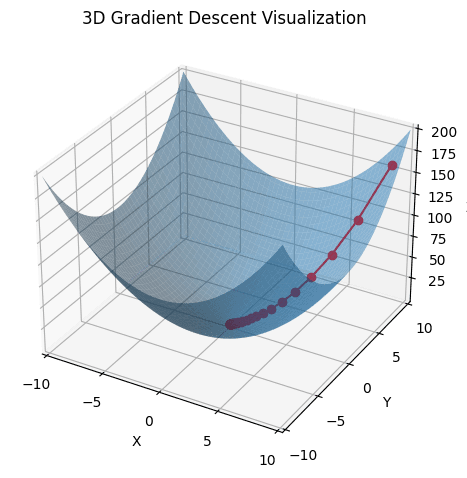

This bowl has a single, global minimum. Real loss surfaces can have local minima where descent gets stuck; random restarts and momentum are two common remedies.

Derivatives and partial derivatives

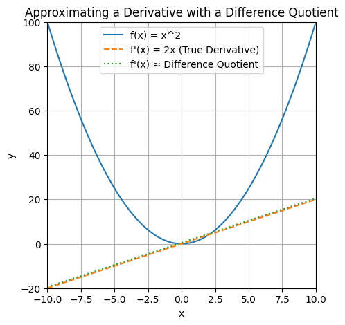
For a function of one variable, the derivative at $x$ is the limit of the difference quotient

as $h \to 0$. The difference quotient is the slope of the secant through $(x, f(x))$ and $(x + h, f(x + h))$; as $h$ shrinks the secant approaches the tangent, whose slope is the derivative. With $h = 0.5$ the approximation to $f'(x) = 2x$ is already close:

A function of several variables has one partial derivative per input: how $f$ changes when only that input changes, the others held fixed. (See the partial derivatives note.) Estimated numerically:

def partial_derivative(f, point, var_idx, h):
    point_plus_h = point.copy()
    point_plus_h[var_idx] += h
    return (f(*point_plus_h) - f(*point)) / h

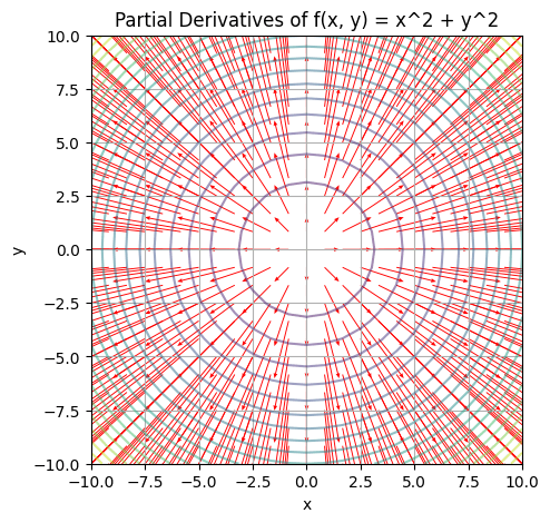
A quiver plot draws the gradient as an arrow at each point. For $f(x, y) = x^2 + y^2$ every arrow points directly away from the minimum at the origin, and the arrows get longer further out, because the function is steeper there:

Choosing the step size

The direction is easy; the size of the step is not. Too small and descent takes forever; too large and it overshoots the minimum, possibly diverging. Options include:

• a fixed step size
• shrinking the step size over time
• at each step, choosing the step size that minimises the objective along that direction (a line search), which works well but costs extra computation per step

Fitting a line

A parameterised model has parameters we can adjust to make its predictions match the data. Take a straight line

and synthetic data from $y = 30x + 7$ for $x$ from −50 to 49, so we know the answer. We want the $m$ and $b$ that minimise the mean squared error:

Write $e_i = y_i - (mx_i + b)$ for the error on point $i$. By the chain rule, the outer square differentiates to $2e_i$, and $e_i$ differentiates to $-x_i$ with respect to $m$ and to $-1$ with respect to $b$ (everything else is a constant, whose derivative is zero). So

In code it is tidier to define the error the other way round, as prediction minus actual, which absorbs the minus signs:

def linear_gradient(x: float, y: float, params: tuple[float, float]) -> list[float]:
    slope, intercept = params
    error = (slope * x + intercept) - y
    return [2 * error * x, 2 * error]
 
 
learning_rate = 0.001
params = random.uniform(-1, 1), random.uniform(-1, 1)
for epoch in range(5001):
    grads = np.array([linear_gradient(x, y, params) for x, y in zip(xs, ys)])
    params = params - learning_rate * grads.mean(axis=0)  # step against the gradient

0 [49.79 -0.13]
1000 [29.999 6.038]
3000 [30.000 6.982]
5000 [30.000 7.000]

The slope converges almost immediately; the intercept takes thousands of epochs, because the $x$ values are large and dominate the gradient. Scaling the inputs would fix that. Linear Regression solves the same problem in closed form.

Minibatch gradient descent

On a large dataset, computing the gradient over every row for every step is too slow. Instead we average the gradient over a random sample, a minibatch, and step after each one:

def minibatches(dataset: np.ndarray, batch_size: int, shuffle: bool = True) -> Iterator[np.ndarray]:
    batch_starts = list(range(0, len(dataset), batch_size))
    if shuffle:
        random.shuffle(batch_starts)
    for start in batch_starts:
        yield dataset[start : start + batch_size]

With batches of 10 the same line is found in about 500 epochs.

Stochastic gradient descent

With a batch size of 1 we step on one example at a time. This is stochastic gradient descent, though the name is often used for minibatch descent too. On this toy problem it converges very quickly. In general, though, the gradient for a single example can be quite different from the gradient for the whole dataset, so the path is noisy, and we lose the speed of vectorised computation.

Adapted from Joel Grus, Data Science from Scratch (2nd edition), chapter 8, and Gradient Descent From Scratch by Arseny Turin.

Original notebook

Tags: Mathematics, Machine Learning