Feature Importance

Both halves of this note follow scikit-learn's own examples, credited at the end.

Impurity-based (MDI) vs permutation importance

A random forest's built-in feature_importances_ measures the mean decrease in impurity (MDI): how much each feature's splits reduced impurity, summed over the trees. It has two weaknesses:

1. It is biased towards high-cardinality features, which offer more possible split points.
2. It is computed on training-set statistics, so a feature the model uses to overfit can look important even if it says nothing about new data.

To show this, take the Titanic data and add two pure-noise columns: random_num, a numeric column with a unique value per row, and random_cat, a categorical column with three values. Fit a fully grown forest: training accuracy is 1.000 and test accuracy 0.814, so it has memorised the training set but still generalises reasonably thanks to bagging.

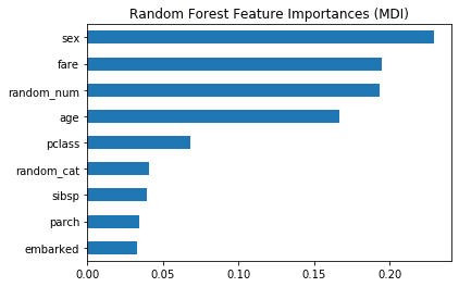
MDI ranks the numeric features highest, including random_num. Its high cardinality explains why it beats random_cat; training-set statistics explain why either gets any importance at all.

Permutation importance instead shuffles one column at a time on held-out data and measures how much the score drops. Shuffling breaks the column's relationship with the target, so a column the model relies on causes a large drop:

result = permutation_importance(rf, X_test, y_test, n_repeats=10, random_state=42, n_jobs=-1)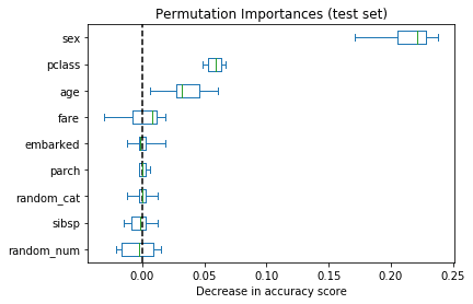

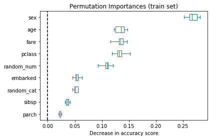
Test set

Training set

On the test set, the low-cardinality sex and pclass matter most and both random columns are near zero. On the training set the random columns rank much higher, which confirms the forest is using them to overfit. Refitting with min_samples_leaf=20 brings training and test accuracy close together, and the random columns lose most of their importance on both sets.

Correlated features

Permutation importance has its own blind spot. If two features are correlated, shuffling one barely hurts, because the model can get the same information from the other. On the Wisconsin breast cancer data a random forest reaches 97% test accuracy, yet no single feature's permutation drops accuracy by more than about 0.012:

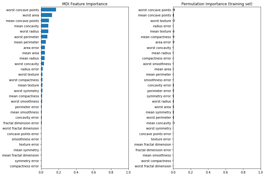
Some feature must matter. The fix is to cluster the features by correlation and keep one from each cluster. That takes a few SciPy pieces.

Spearman's rank correlation

scipy.stats.spearmanr replaces each value by its rank and computes Pearson's correlation on the ranks. That captures any monotonic relationship, not just linear ones. Without ties it reduces to

where $d_i$ is the difference between the two ranks of observation $i$; with ties, only the Pearson-on-ranks definition is exact. Given a 2-D array it returns a symmetric correlation matrix with ones on the diagonal, plus a matrix of p-values.

Distances: squareform and pdist

scipy.spatial.distance.squareform converts between a full, symmetric distance matrix (zeros on the diagonal) and a condensed 1-D form that keeps each pair once. The condensed form is the upper triangle, read row by row:

squareform(np.array([[0, 1, 2], [1, 0, 3], [2, 3, 0]]))  # array([1, 2, 3])

pdist computes the condensed distances between every pair of rows of an array, Euclidean by default. $n$ rows give $n(n-1)/2$ distances, so the output grows quadratically.

Ward linkage and dendrograms

scipy.cluster.hierarchy.ward performs agglomerative clustering, at each step merging the two clusters whose union increases total within-cluster variance the least. It returns a linkage matrix with $n - 1$ rows, one per merge:

• Columns 0 and 1: the two clusters merged. Indices below $n$ are original observations; index $n + i$ is the cluster formed at step $i$.
• Column 2: the distance between them, here the Ward merge cost.
• Column 3: the number of observations in the new cluster.

A dendrogram draws these merges as a tree. Leaves are observations, each internal node is a merge, and its height is the merge distance.

Putting it together

Turn the correlation matrix into a distance (1 − |correlation|), cluster it, and cut the tree at a threshold chosen by eye from the dendrogram:

corr = spearmanr(X).correlation
corr = (corr + corr.T) / 2
np.fill_diagonal(corr, 1)
dist_linkage = hierarchy.ward(squareform(1 - np.abs(corr)))
 
cluster_ids = hierarchy.fcluster(dist_linkage, 1, criterion="distance")
cluster_id_to_feature_ids = defaultdict(list)
for idx, cluster_id in enumerate(cluster_ids):
    cluster_id_to_feature_ids[cluster_id].append(idx)
selected_features = [X.columns[v[0]] for v in cluster_id_to_feature_ids.values()]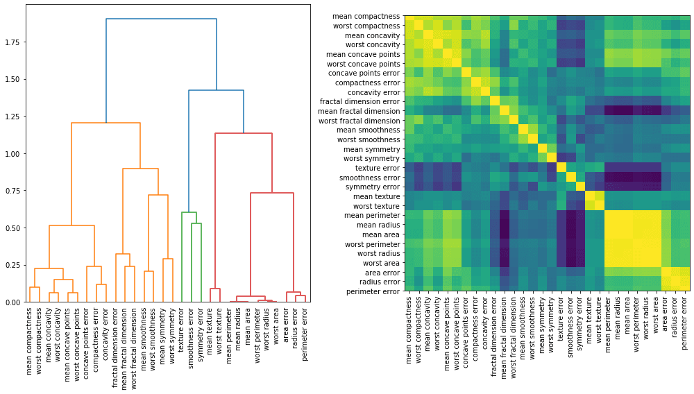

The size-related features (radius, perimeter, area and their variants) form one tight cluster, as we'd expect. Keeping one feature per cluster leaves five, and test accuracy stays at 0.97:

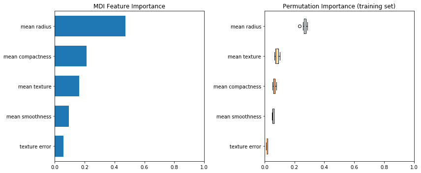
Mean radius is now clearly the most important feature. Before, the size features were substitutes for each other, so permuting any one of them cost almost nothing, and each looked unimportant even though size as a whole mattered most.

Sources

• Permutation importance vs random forest feature importance (MDI), scikit-learn
• Permutation importance with multicollinear or correlated features, scikit-learn

Original notebook

Tags: Machine Learning