Gain, Lift and Deciles

Updated 1st November 2026Started 18th February 2023

These curves answer a practical question: if we act on the rows the model ranks highest, how many of the positives do we reach? They use the same Titanic random forest as Classification Metrics. In the test set 38% of passengers survived, so survival is the positive class.

Gain

Sort the rows by predicted probability, highest first. The gain for the top fraction of rows is the share of all positives found there:

\text{gain} = \frac{\text{positives in the subset}}{\text{positives in the whole sample}}

A perfect model would find every survivor in the top 38% of rows, for 100% gain. A real model has false positives near the top, so it takes more than 38% of the rows to get there, and 100% gain only arrives at the end, because some survivors get very low predicted probabilities. Random selection gives gain equal to the fraction of rows taken. This is the same cumulative curve as the CAP chart, just with both axes as proportions.

Lift

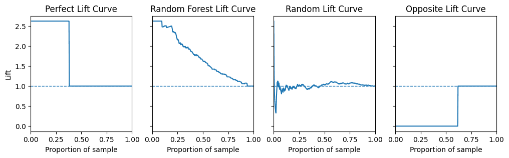
Lift compares the positive rate in the top fraction with the positive rate overall:

\text{lift} = \frac{\text{positives in the subset} \;/\; \text{rows in the subset}}{\text{positives in the sample} \;/\; \text{rows in the sample}}

Equivalently, lift is gain divided by the fraction of rows taken. Random selection has a lift of 1. With 38% positives the highest possible lift is $1 / 0.38 = 2.63$ , which a perfect model would hold across its top 38% of rows.

def plot_lift(y_proba, y_real, ax=None):
    df = pd.DataFrame({"y_real": y_real, "y_proba": y_proba}).sort_values("y_proba", ascending=False)
    total_positive_ratio = (df["y_real"] == 1).mean()
    lift_values = []
    for threshold in df["y_proba"]:
        subset = df[df["y_proba"] >= threshold]
        lift_values.append((subset["y_real"] == 1).mean() / total_positive_ratio)
    ...

Gain and lift curves for the Titanic random forest

Decile analysis

Decile analysis is the tabular version, common in marketing and credit risk: sort by predicted probability, cut into ten equal groups, and count the positives in each. Decile 1 is the group the model rates most likely, for example to respond to an advert or default on a loan.

df = pd.DataFrame({"y_proba": preds_test, "y_real": y_test}).sort_values("y_proba", ascending=False)
df = df.reset_index(drop=True)
df["decile"] = pd.qcut(df.index, 10, labels=False) + 1

Decile	Rows	Positives	Positive rate	Gain	Lift	Probability range
1	33	32	0.97	0.26	2.54	0.95 to 1.00
2	33	29	0.88	0.49	2.43	0.83 to 0.95
3	33	16	0.48	0.62	2.04	0.64 to 0.81
4	32	15	0.47	0.74	1.84	0.45 to 0.63
5	33	11	0.33	0.82	1.65	0.28 to 0.45
6	33	5	0.15	0.86	1.44	0.19 to 0.28
7	32	6	0.19	0.91	1.31	0.11 to 0.19
8	33	4	0.12	0.94	1.18	0.05 to 0.11
9	33	3	0.09	0.97	1.08	0.02 to 0.05
10	33	4	0.12	1.00	1.00	0.00 to 0.02

Gain and lift here are cumulative: the top two deciles hold 49% of the survivors, at 2.43 times the base rate. A well-ranked model has positive rates that fall steadily down the table; the small rise in decile 10 shows a few survivors the model was confidently wrong about.

Sources

Code adapted from vinyluis/Articles: Decile, Gain, Lift
The lost art of decile analysis
scikit-plot draws these curves out of the box

Original notebook

Linked from

Classification Metrics

Revision log

1st November 2026Migrated from data-science-notes; fixed the lift formula

Tags: Machine Learning