Drift

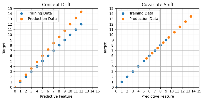
Drift is when the patterns in the training data no longer hold once a model is in production. Given a data-generating process $y = f(x)$, there are two main kinds:

• Concept drift: the relationship between inputs and target changes, i.e. $f$ (more precisely $P(y \mid x)$) changes.
• Covariate shift: the distribution of the inputs, $P(x)$, changes, while the relationship stays the same.

Detecting drift

Three ways:

• Monitor descriptive statistics of the data over time, for example with the population stability index.
• Backtest: train on one period and validate on a later one.
• Use domain knowledge to anticipate when things are about to change.

The example uses the Grupo Bimbo bakery data from the dynamic decisions note.

Compositional change

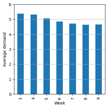
Gaps in the data change its composition over time. Restricting to a single product (ID 1238) still leaves the number of locations stocking it falling every week, from 194,927 rows in week 3 to 154,140 in week 9. Three quarters of store and client combinations have 5 weeks of records or fewer. Keeping only those with all 7 weeks removes most of the compositional change, and shows average demand falling from about 5.4 to about 4.6.

Before filtering gaps away, it is worth asking whether they carry signal (a product being withdrawn), are noise, or can be corrected for.

Backtesting

Train one model per week and validate each on the following week. If every model does about as well, there is little sign of drift. If performance varies a lot, the validation score of a model trained on everything is a poor guide to how it will do in future.

data = data.sort_values("Semana").reset_index(drop=True)
for training_week in weeks[1:-1]:  # week 3 has no previous week to lag from
    val_week = training_week + 1
    train_index = data[data["Semana"] == training_week].index
    val_index = data[data["Semana"] == val_week].index
    for seed in [0, 1, 2]:
        model, val_loss = train(dataset(train_index), dataset(val_index), seed=seed)
        metrics.append({"training_week": training_week, "seed": seed, "val_mse": val_loss})

The features are last week's demand, units sold and returns for each store and client, so the model only sees what it would know when ordering. Three seeds per week show how much of any difference is just training noise, and forecasting last week's demand gives a baseline.

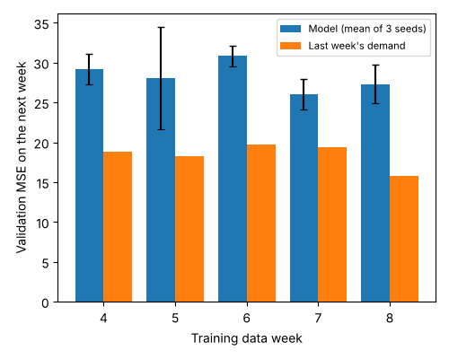
No week stands out. The model's validation MSE moves between 26 and 31, which is about the size of the variation between seeds (a standard deviation of up to 6.4 for week 5). So this backtest finds no sign of drift in the relationship, even though average demand fell steadily. The model is also 7 to 12 MSE worse than the naive baseline in every week, which is the more useful finding.

This replaces the original backtest, which showed one week (training on week 3) with far higher loss than the others. That result was not drift. The model used the same week's units sold as a feature, which nearly gives away the target, and the code indexed the sorted arrays with the unsorted DataFrame's index labels, so training and validation rows were mismatched. Each bar was also a single training run.

Responding to covariate shift

Covariate shift does not change the relationship, but the model is now predicting in a region where it saw less data. Update the simulation to match: if more high-income customers are coming and they are known to buy more often, build that into the simulated population.

Responding to concept drift

The example is the Telco churn dataset with an XGBoost classifier in a scikit-learn pipeline (one-hot encode the categorical columns, pass the numeric ones through).

Adjusting predictions for a segment

Suppose market news suggests DSL customers are about to churn more than history implies. The simplest response is to adjust their predictions directly:

def prediction_adjust_DSL(data):
    baseline = pipeline.predict_proba(data[cols_to_use])[:, 1]
    has_DSL = data["InternetService"] == "DSL"
    return np.clip(baseline + has_DSL * 0.1, 0, 1)

Note this adds 10 percentage points, not 10%. The number is arbitrary. Even without a strong justification for a particular size, nudging predictions in the direction you expect the business to move is often better than ignoring the expectation.

Adjusting a feature's effect with SHAP

Instead of adjusting a segment, you can shrink how much one feature contributes. SHAP splits each prediction into per-feature contributions, so you can subtract part of one feature's contribution. Here, halving the effect of tenure:

from scipy.special import expit
 
preprocessor = pipeline.named_steps["preprocessor"]
classifier = pipeline.named_steps["classifier"]
explainer = shap.TreeExplainer(classifier, data=preprocessor.transform(X_train[cols_to_use]))
feature_names = list(preprocessor.get_feature_names_out())
tenure_column = feature_names.index("remainder__tenure")
 
def prediction_with_less_effect_for_tenure(data, reduction=0.5):
    encoded = preprocessor.transform(data[cols_to_use])
    log_odds = classifier.predict(encoded, output_margin=True)
    shap_values = explainer.shap_values(encoded)
    return expit(log_odds - reduction * shap_values[:, tenure_column])

The original version had two bugs, and they hid each other:

1. Units. For an XGBoost classifier, TreeExplainer explains the raw output, which is in log-odds. The original subtracted those log-odds contributions from probabilities and clipped to $[0, 1]$. The adjustment has to happen in log-odds, then go back through the sigmoid, as above.
2. Column. It used column 0 as tenure. But ColumnTransformer puts transformed columns first and the passthrough remainder last, so column 0 was the first one-hot column (from PhoneService), and tenure was second from last. Looking the index up by name avoids this.

As a result the original plot showed the "tenure" adjustment barely moving the predictions, which should itself have been a warning: tenure is one of the strongest churn predictors in this data. Plot the adjusted and baseline prediction distributions, and check how the change interacts with the business decision, before putting anything like this into production.

Sim2Real

How do you make sure a simulation is useful in the real world?

• Make it better.
• Treat it like overfitting: simpler decision rules are likely to be more robust.
• Validate it with people close to the existing process.
• Test on a small scale first, for example with an A/B test.

A good test randomises while keeping contamination low, and the two pull against each other. Discounts for a random set of customers everywhere may annoy the customers who see others getting them. Discounting a whole region instead avoids that, but there are far fewer regions than customers, so there is much less randomisation. Switching a store's decision rule at random week to week fails if last week's rule affects this week's behaviour, as it does with carried-over stock.

The loop is: simulate, choose a decision rule, test, and feed what you learn back into the simulation.

Adapted from Dan Becker's Machine Learning for Business Decision Optimization course.

Original notebook

Tags: Machine Learning, Decision Optimisation