Dynamic Decisions
In a static decision, what you choose this period does not affect what you face next period. If stock perishes before the next order arrives, each order can be optimised on its own, as in continuous outcomes.
In a dynamic decision, the action feeds back into the state. An agent (us, or our code) sees a state and takes an action, such as placing an order. The environment (this week's demand) produces a reward, and also the next state: surplus stock carried into next week.
When is dynamic optimisation worth it?
Simulation is much more work than a static model, so ask:
- One-shot or connected? The main question: does today's decision change tomorrow's situation?
- Certain or uncertain long-term payoffs? If you know what each decision will pay, a static model may do.
- Immediate or delayed payoffs? Decisions can be technically sequential but pay off so soon that a static model is fine.
Some examples:
- Telecom churn: mostly static, though whether to discount someone next month or the month after is a sequential question.
- Retail inventory: dynamic, unless all stock perishes before the next order.
- Hotel pricing: dynamic. A room not sold today can still be sold later, perhaps at a different price.
- Credit underwriting: often static, but a repeat relationship with a customer adds a dynamic element.
The data
The Grupo Bimbo inventory demand dataset has weekly sales of bakery products for weeks 3 to 9, keyed by store (Agencia_ID), channel, route, client and product. The target is Demanda_uni_equil, adjusted demand.
Most ID combinations do not appear every week (the median appears in 2 of 7). In a real project you would find out why: missing data, products launched or retired, or genuinely zero sales. Here we keep only combinations present in all 7 weeks, which leaves 17.6 million rows.
The model is a small PyTorch network with an embedding for each ID column, as in the PyTorch note. Week 4 trains it, and weeks 5 to 9 are used to compare decision rules.
Fixing a leak
The original notebook fed the model Venta_uni_hoy and Venta_hoy, the units sold and sales value in the same week as the demand being predicted. Adjusted demand is essentially units sold minus returns, so the model was reading the answer off its inputs, and scored an R² of 0.994. You do not know this week's sales when you place this week's order.
The version here uses only what is known before ordering: last week's demand, units sold and units returned for the same ID combination. Week 3 has no previous week, so training moves to week 4 (a 500,000-row sample, split 80/20 as before). The result:
| Model | Validation R² | Validation MSE |
|---|---|---|
| Original, with same-week sales (leaky) | 0.994 | 7.5 |
| Lagged features only | 0.786 | 293.9 |
| No model: forecast last week's demand | 0.795 | 281.3 |
Without the leak, the network does no better than simply repeating last week's demand. That is worth knowing before building anything more elaborate, and it is a reminder to always compare against a naive baseline. The large MSE comes from a few combinations with very high demand.
Because the decisions do not change what customers want to buy, the predictions can be computed up front, before the simulation runs. (One caveat: recorded demand may be capped by what the shop had in stock, which would make it partly a consequence of past decisions.)
The simulation
The heart of it is a loop over weeks, where each week starts with whatever was left over from the last. The assumptions:
- Old stock sells before new stock.
- Old stock not sold this week spoils.
- Only unsold new stock carries over, so leftover stock is between 0 and the amount of new stock.
def create_simulation_table(actual_demand, forecasted_demand, decision_rule):
    df = pd.DataFrame()
    weeks = range(1, len(actual_demand) + 1)
    for week, actual, forecast in zip(weeks, actual_demand, forecasted_demand):
        df.loc[week, "actual_demand"] = actual
        df.loc[week, "predicted_demand"] = forecast
        df.loc[week, "old_stock"] = 0 if week == 1 else df.loc[week - 1, "leftover_stock"]
        df.loc[week, "new_stock"] = decision_rule(df.loc[week])
        old, new = df.loc[week, "old_stock"], df.loc[week, "new_stock"]
        df.loc[week, "actually_sell"] = min(actual, old + new)
        df.loc[week, "shortage"] = actual - df.loc[week, "actually_sell"]
        df.loc[week, "spoiled"] = max(old - actual, 0)
        df.loc[week, "leftover_stock"] = max(0, min(old + new - actual, new))
    return df
With dummy demand of 5, 7, 3, 1, 6, forecasts of 7, 3, 2, 4, 1, and a rule of "order 10% more than the forecast, rounded up":
| Week | Demand | Forecast | Old stock | New stock | Sold | Shortage | Spoiled | Leftover |
|---|---|---|---|---|---|---|---|---|
| 1 | 5 | 7 | 0 | 8 | 5 | 0 | 0 | 3 |
| 2 | 7 | 3 | 3 | 4 | 7 | 0 | 0 | 0 |
| 3 | 3 | 2 | 0 | 3 | 3 | 0 | 0 | 0 |
| 4 | 1 | 4 | 0 | 5 | 1 | 0 | 0 | 4 |
| 5 | 6 | 1 | 4 | 2 | 6 | 0 | 0 | 0 |
Week 2 shows the dynamic part: a forecast of 3 would have left us short, but the 3 units carried over from week 1 covered it.
Comparing decision rules
To score a rule we need an objective. This one is illustrative, not derived from real costs: each unit sold is worth 1, each unit of unmet demand costs 3, and spoiled and carried-over stock cost 0.5 each.
def objective_function(df):
    return (
        df["actually_sell"].sum()
        - 3 * df["shortage"].sum()
        - 0.5 * df["spoiled"].sum()
        - 0.5 * df["old_stock"].sum()
    )
Four rules:
def predicted_need(state):
    return max(0, np.ceil(state["predicted_demand"] - state["old_stock"]))

def predicted_need_plus_one(state):
    return predicted_need(state) + 1

def predicted_need_plus_two(state):
    return predicted_need(state) + 2

def predicted_demand(state):
    return np.ceil(state["predicted_demand"])
The original predicted_need had no max(0, ...), so whenever old stock exceeded the forecast it placed a negative order. Predictions are also clipped at zero.
The rules are compared on store 1110, with store 24049 held back to test the winner:
| Rule | Shortages (count) | Total shortage | Sold | Old stock | Spoiled | Objective |
|---|---|---|---|---|---|---|
predicted_need | 5,477 | 65,178 | 277,939 | 66,806 | 15,205 | 41,400 |
predicted_need_plus_one | 4,672 | 59,437 | 283,680 | 72,942 | 16,809 | 60,494 |
predicted_need_plus_two | 3,993 | 54,504 | 288,613 | 79,693 | 18,726 | 75,892 |
predicted_demand | 4,347 | 50,371 | 292,746 | 125,839 | 37,428 | 60,000 |
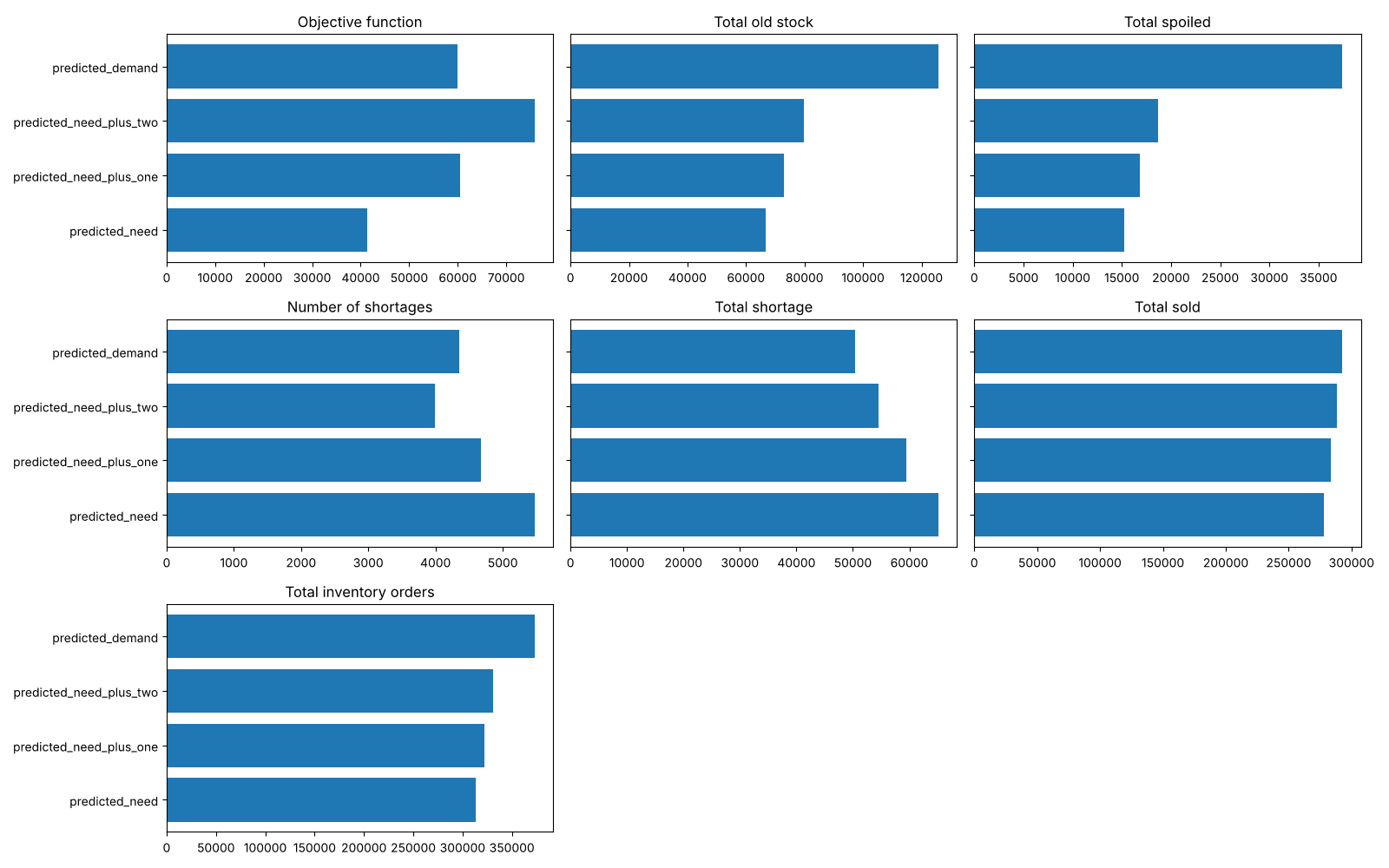
What this shows:
- An honest forecast changes the picture. With the leaky model, shortages and spoilage were tiny and every rule scored about 277,000 to 298,000. With a realistic forecast, shortages are 3 to 6 times higher, spoilage is 60 to 145 times higher, and the objective falls by 78 to 85%.
predicted_demandignores what is carried over, so it orders the most, carries the most old stock and spoils twice as much as any other rule. It has the fewest units short, but it still loses to the buffered rules.- Buffers pay. Each extra unit of buffer cuts shortages, and because the objective weights a unit short six times as heavily as a unit of old stock, the objective keeps rising up to
predicted_need_plus_two. With a forecast this noisy, the buffer is doing a lot of the work.
On the held-back store, predicted_need_plus_two also beats predicted_need (5,363 against −16,882), though the objective there is barely positive. Whether the weights in the objective are right depends on the business. Once you trust the simulation, the size of the buffer can be tuned with any hyperparameter search tool, then checked on the held-back store.
Next: drift, and what happens when the patterns in the simulation stop holding.
Adapted from Dan Becker's Machine Learning for Business Decision Optimization course.
Linked from
Revision log
- Migrated from data-science-notes; retrained without the leaky same-week features and reran the rule comparison
Tags: Machine Learning, Decision Optimisation