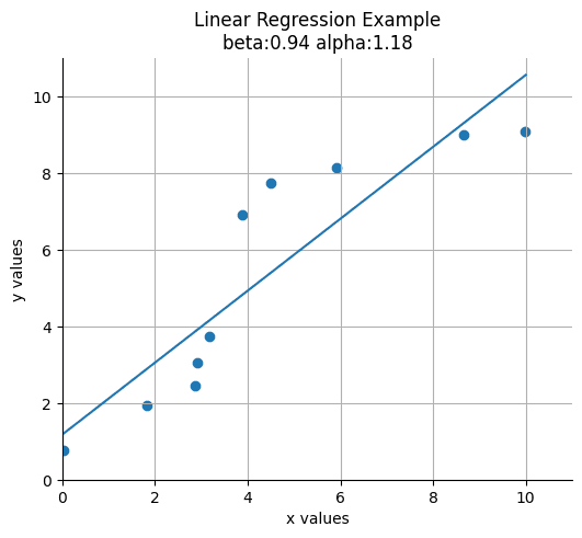
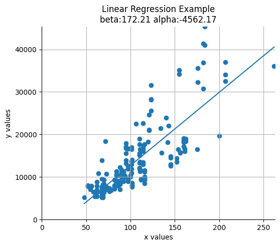
Correlation tells us how strong a linear relationship is. Linear regression lets us use it: given a house's size, predict its price.
One independent variable
We hypothesise a linear model
yi=βxi+α
where yi is the price of house i, xi its size, β the slope and α the intercept. Least squares picks the α and β that minimise the sum of squared errors (residuals), our cost function S:
S=i=1∑n(yi−y^i)2=i=1∑n(yi−α−βxi)2
At the minimum, the partial derivatives of S with respect to α and β are both zero. (The chain rule and partial derivatives notes cover the calculus.)
Finding α
Differentiating with the chain rule, with u=yi−α−βxi: the outer u2 becomes 2u, and the inner term differentiates to −1 with respect to α. Setting the result to zero:
0=i=1∑n−2(yi−α−βxi)
Dividing by −2 and splitting the sum, with ∑i=1nα=nα:
Gradient Descent fits the same line numerically instead of in closed form.
Multiple regression
With several independent variables, for example minutes a data scientist spends on a social network:
minutes=β1friends+β2work hours+β3has PhD+α
the single number xi becomes a vector xi1,…,xik:
yi=β1xi1+⋯+βkxik+α
and the parameters become a vector β. We assume the columns of x are linearly independent: no column can be written as a weighted sum of the others. Otherwise the coefficients are not uniquely determined.
Derivation adapted from Linear Regression Intuition by Ridley Leisy; multiple regression from Joel Grus, Data Science from Scratch, chapter 15.