Logistic Regression
Regression models predict a continuous quantity, and a probability is one. A probability-predicting model becomes a classifier once we add a decision rule, such as "if the probability is 50% or more, call it a cat".
Logistic regression predicts probabilities, so strictly it is a regression method, even though machine learning usually files it under classification because that is what it is mostly used for. Methods like SVMs are classifiers in the stricter sense: they predict an outcome without a probability.
In scikit-learn:
X = np.array([[1, 1], [1, 2], [1, 3], [1, 4], [1, 5]])  # first column is a constant, for the intercept
y = np.array([0, 0, 0, 1, 1])

model = LogisticRegression(random_state=0).fit(X, y)
model.predict_proba(X)[:, 1]  # [0.063, 0.161, 0.353, 0.608, 0.816]
model.predict(X)              # [0, 0, 0, 1, 1]
Odds
The odds of an event are the probability it happens over the probability it doesn't:
| Event | Probability | Odds |
|---|---|---|
| Heads | 1/2 | 1, or 1:1 |
| Rolling 1 or 2 | 1/3 | 1/2, or 1:2 |
| Drawing a diamond | 1/4 | 1/3, or 1:3 |
From a linear model to a probability
The outcome follows a Bernoulli distribution (a binomial with one trial): 1 with some unknown probability , 0 with probability . The goal is to estimate for any combination of the independent variables.
A linear combination of the variables,
can take any real value, so we need a link between the real line and the interval . The logit, the natural log of the odds, maps onto the whole real line:
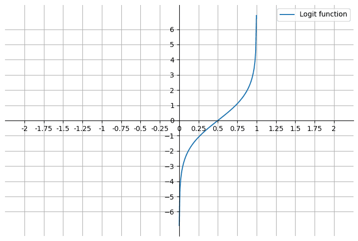
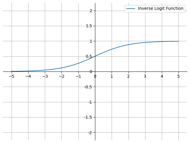
That has the probabilities on the x axis; we want them as the output. So set the logit equal to and invert:
This is the sigmoid or logistic function . It maps any real input into the open interval , never quite reaching 0 or 1.
Fitting by maximum likelihood
The coefficients are usually found by maximum likelihood estimation. The likelihood of a coefficient vector is the product of the predicted probabilities of what actually happened:
where is the feature vector of observation , its outcome, and the predicted probability of the positive class.
A product of many small numbers underflows, so we maximise the log-likelihood instead:
There is no closed-form solution, so we climb it iteratively. The sigmoid's derivative, , makes the gradient come out neatly:
That is, the error for each observation, weighted by its features and summed. The transpose is what makes the shapes line up: is and the error is , so (which is ) times the error gives one gradient entry per weight.
From scratch
- Start with all weights at zero.
- Compute scores (one weighted sum per row) and pass them through the sigmoid.
- Subtract the predictions from the labels to get the error.
- Take a step up the gradient (gradient ascent, since we are maximising), scaled by the learning rate.
def sigmoid(x):
    return 1 / (1 + np.exp(-x))


def predict_proba(x, weights):
    return sigmoid(np.dot(x, weights))


def logistic_regression(X, y, num_steps: int, learning_rate: float):
    weights = np.zeros(X.shape[1])
    for step in range(num_steps):
        error = y - predict_proba(X, weights)
        gradient = np.dot(X.T, error)
        weights += learning_rate * gradient
    return weights


weights = logistic_regression(X, y, num_steps=1_000_000, learning_rate=5e-5)
predict_proba(X, weights)  # [0.002, 0.024, 0.248, 0.817, 0.984]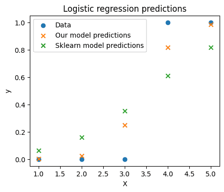
Both models classify all five points correctly, but ours is much more confident. That is not a bug: scikit-learn's LogisticRegression applies L2 regularisation by default (C=1.0), which shrinks the coefficients and pulls the probabilities towards 0.5. With penalty=None, or a very large C, it matches the from-scratch fit. With data this cleanly separable the unregularised optimum is at infinity, so our weights depend on how long we run.
Why not linear regression?
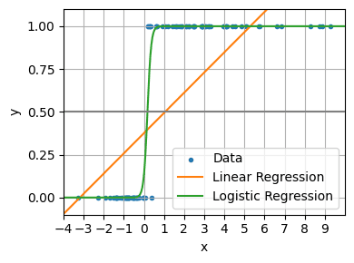
A linear model treats the classes as the numbers 0 and 1 and fits the best straight line through them. That line is not a probability: it goes below 0 and above 1, and a few extreme values tilt it badly. Logistic regression stays bounded and behaves at both extremes.
Interpreting coefficients: the odds ratio
An odds ratio compares two odds. A loaded coin that lands heads 70% of the time has odds ; a fair coin has odds 1. So the odds ratio of heads, loaded against fair, is
In logistic regression, is the odds ratio for a one-unit increase in , holding the other variables constant. Take a fictitious model of sleep apnoea against body weight, where weight has an odds ratio of 1.07:
- Each extra pound multiplies the odds of apnoea by 1.07, a 7% increase.
- Ten extra pounds multiply them by , nearly doubling the odds.
- This holds at any point on the weight scale. It is the odds that change by a constant factor, not the probability.
Linked from
Revision log
- Migrated from data-science-notes; fixed the likelihood notation and odds ratio wording
Tags: Statistics, Machine Learning