Bayesian Data Analysis
Bayesian data analysis takes a question in the form of a model and uses logic to produce an answer in the form of probability distributions. At its simplest:
- For each possible explanation of the data, count all the ways the data could happen.
- Explanations with more ways to produce the data are more plausible.
Marbles in a bag
A bag holds four marbles, each blue (B) or white (W), in unknown proportion. There are five possible bags, our conjectures: WWWW, BWWW, BBWW, BBBW and BBBB.
We draw three marbles, with replacement, and see B W B. Which bag is it?
For each conjecture, count the ways it could produce that sequence: the number of blue marbles, times the number of white, times the number of blue. (McElreath draws these counts as a "garden of forking paths", one ring per draw.)
| Conjecture | Ways to produce B W B | Plausibility |
|---|---|---|
| WWWW | 0 × 4 × 0 = 0 | 0 |
| BWWW | 1 × 3 × 1 = 3 | 0.15 |
| BBWW | 2 × 2 × 2 = 8 | 0.40 |
| BBBW | 3 × 1 × 3 = 9 | 0.45 |
| BBBB | 4 × 0 × 4 = 0 | 0 |
The plausibilities are just the counts normalised to sum to 1. The rules for Bayesian updating:
- State a causal model for how observations arise, given each possible explanation.
- Count the ways the data could arise under each explanation.
- The relative plausibility of each explanation is its relative count.
Updating
Now we draw another B. The new draw is independent of the earlier ones, so we can take the previous counts as our prior and multiply each by the number of ways that conjecture produces the new observation:
| Conjecture | Ways to produce B | Previous count | New count | New plausibility |
|---|---|---|---|---|
| WWWW | 0 | 0 | 0 × 0 = 0 | 0 |
| BWWW | 1 | 3 | 3 × 1 = 3 | 0.07 |
| BBWW | 2 | 8 | 8 × 2 = 16 | 0.35 |
| BBBW | 3 | 9 | 9 × 3 = 27 | 0.59 |
| BBBB | 4 | 0 | 0 × 4 = 0 | 0 |
Each updated set of plausibilities becomes the prior for the next observation. The process also runs backwards: knowing the final plausibilities and that the last draw was B, we could divide that observation back out. So the order in which the data arrive doesn't matter, and presenting it all at once is just a shortcut for the same iterated process.
Some consequences:
- There is no minimum sample size. With little data the posterior is flat and wide, but it is still a valid statement of what we know.
- The shape of the posterior embodies the sample size: more data makes it narrower and taller.
- Point estimates matter less, because the estimate is the distribution. Summarise only at the end; summarising earlier throws away uncertainty.
- Intervals are fine as summaries, but there is nothing special about any particular width, such as 95%.
How much of the globe is water?
We toss an inflatable globe nine times and record whether our right index finger lands on water (W) or land (L):
Six waters in nine tosses. If each toss lands on water with probability , the counts are binomial:
Written as a model, with a flat prior on :
Grid approximation
The simplest way to get the posterior is to evaluate prior × likelihood on a grid of candidate values of , then normalise:
def posterior_grid_approx(grid_points: int = 5, success: int = 6, tosses: int = 9):
    p_grid = np.linspace(0, 1, grid_points)
    prior = np.repeat(1, grid_points)  # uniform
    likelihood = stats.binom.pmf(success, tosses, p_grid)
    unstd_posterior = likelihood * prior
    posterior = unstd_posterior / unstd_posterior.sum()
    return p_grid, posterior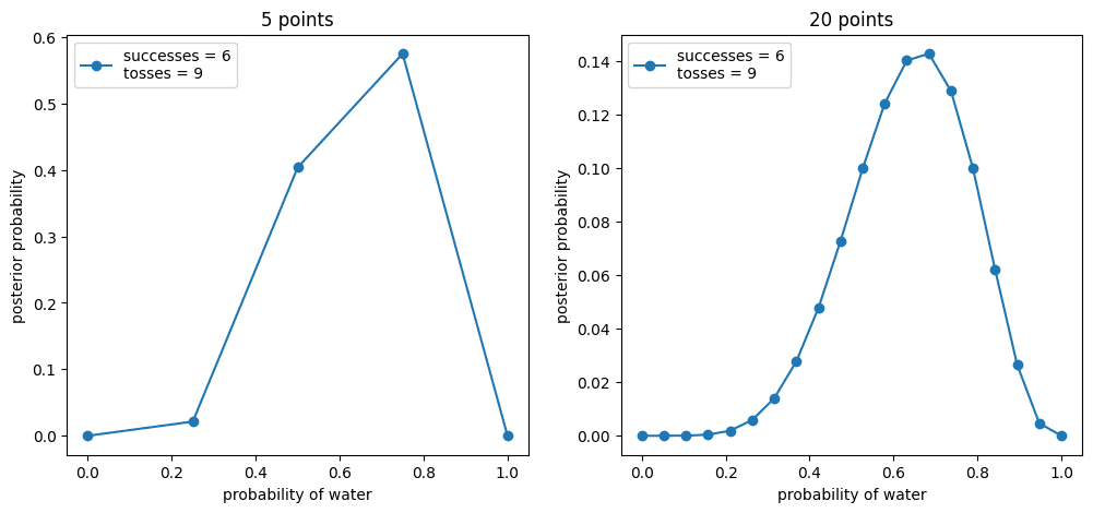
Five grid points give a crude sketch; twenty already show the shape, peaking a little below 0.7.
Adapted from Richard McElreath, Statistical Rethinking (2nd edition), chapters 1 and 2.
Linked from
Revision log
- Merged the two copies from data-science-notes; corrected the updated plausibilities
Tags: Statistics