Probability

Dependence and conditional probability

$P(E)$ is the probability of event $E$. Events $E$ and $F$ are dependent if knowing whether $E$ happened tells us something about whether $F$ happened, and independent otherwise. Independence is exactly the condition that the probability of both is the product of each:

In general, provided $P(F) > 0$, the probability of $E$ given $F$ is

and when $E$ and $F$ are independent this reduces to $P(E \mid F) = P(E)$.

Two children

A family has two children, each equally likely to be a boy or a girl. What is the probability both are girls, given that the older one is a girl? The event "both are girls and the older is a girl" is just "both are girls", so

Now condition instead on "at least one is a girl". Of the four equally likely families (GG, GB, BG, BB) three qualify, and only one of those is GG:

Knowing only that at least one child is a girl, a boy-and-girl family is twice as likely as two girls.

Bayes' theorem

Bayes' theorem reverses a conditional probability. Using the definition twice:

$F$ splits into the mutually exclusive events "$F$ and $E$" and "$F$ and not $E$", so the denominator can be expanded:

A disease affects 1 in 10,000 people. A test detects it 99% of the time when it is present, and gives a false positive 1% of the time when it is not. Given a positive test:

Under 1%. In natural frequencies: of a million people, 100 have the disease and 99 of them test positive; of the 999,900 who don't, 9,999 test positive. So only 99 of the 10,098 positives are real.

This assumes people are tested at random. If only people with symptoms take the test, we should condition on "positive and symptomatic", and the answer would be much higher.

Random variables

A random variable is a variable whose possible values have a probability distribution. Its expected value is the average of its values weighted by their probabilities:

• A coin flip that is 1 for heads and 0 for tails has expected value $0 \times \frac{1}{2} + 1 \times \frac{1}{2} = \frac{1}{2}$.
• The number of heads in 10 flips has expected value 5.
• A number drawn uniformly from range(10) (0 to 9) has expected value 4.5.

Random variables can be conditioned on events too. Let $X$ be the number of girls in the two-child example: 0 with probability $\frac{1}{4}$, 1 with probability $\frac{1}{2}$, 2 with probability $\frac{1}{4}$. Conditioned on at least one girl, it is 1 with probability $\frac{2}{3}$ and 2 with probability $\frac{1}{3}$. Conditioned on the older child being a girl, it is 1 or 2 with probability $\frac{1}{2}$ each.

Continuous distributions

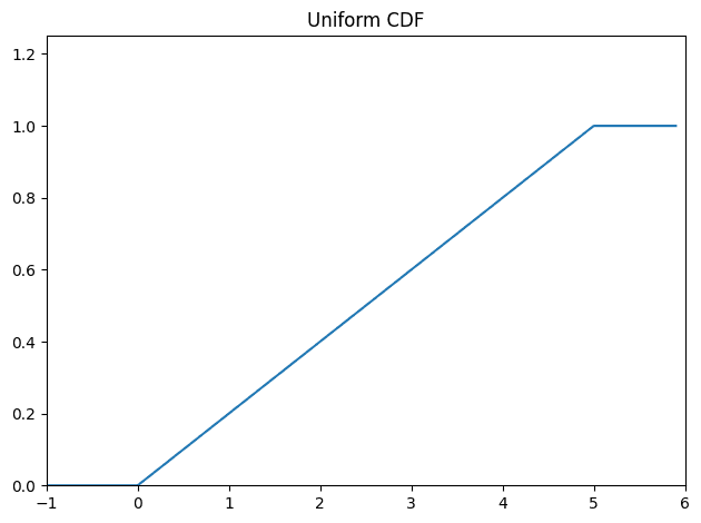
A discrete distribution puts positive probability on individual outcomes. Over a continuum there are infinitely many points, so each individual point has probability zero. Instead we use a probability density function (PDF): the probability of a value falling in an interval is the integral of the density over that interval. The cumulative distribution function (CDF) gives the probability that the variable is less than or equal to a value.

Uniform distribution

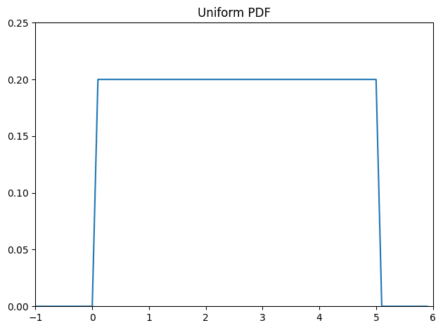
The uniform distribution on $[a, b]$ puts equal density on every value in the interval:

Normal distribution

The normal distribution is symmetric about its mean $\mu$, with spread set by its standard deviation $\sigma$:

def normal_pdf(x: float, mu: float = 0, sigma: float = 1) -> float:
    return math.exp(-((x - mu) ** 2) / 2 / sigma**2) / (math.sqrt(2 * math.pi) * sigma)

With $\mu = 0$ and $\sigma = 1$ it is the standard normal. If $Z$ is standard normal then $X = \sigma Z + \mu$ is normal with mean $\mu$ and standard deviation $\sigma$; conversely $Z = \frac{X - \mu}{\sigma}$ standardises $X$.

The CDF has no elementary closed form, but can be written with the error function:

def normal_cdf(x: float, mu: float = 0, sigma: float = 1) -> float:
    return (1 + math.erf((x - mu) / math.sqrt(2) / sigma)) / 2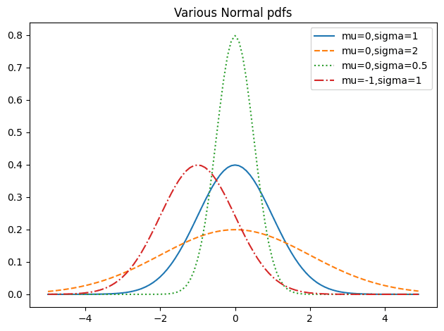

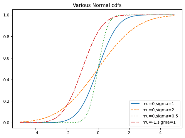
Its inverse has no simple form either, but normal_cdf is continuous and strictly increasing, so a binary search finds it:

def inverse_normal_cdf(p: float, mu: float = 0, sigma: float = 1, tolerance: float = 0.00001) -> float:
    if mu != 0 or sigma != 1:
        return mu + sigma * inverse_normal_cdf(p, tolerance=tolerance)
    low_z, hi_z = -10.0, 10.0
    while hi_z - low_z > tolerance:
        mid_z = (low_z + hi_z) / 2
        if normal_cdf(mid_z) < p:
            low_z = mid_z
        else:
            hi_z = mid_z
    return mid_z

The normal distribution also underlies Student's t-distribution, which describes the standardised sample mean when $\sigma$ has to be estimated from the sample.

The central limit theorem

The average of a large number of independent, identically distributed random variables is approximately normally distributed. If $x_1, \ldots, x_n$ each have mean $\mu$ and standard deviation $\sigma$, then for large $n$

A $\text{Binomial}(n, p)$ variable is the sum of $n$ independent $\text{Bernoulli}(p)$ variables, each 1 with probability $p$. A Bernoulli has mean $p$ and standard deviation $\sqrt{p(1-p)}$, so for large $n$ the binomial is approximately normal with $\mu = np$ and $\sigma = \sqrt{np(1-p)}$. Here are 10,000 draws from $\text{Binomial}(100, 0.75)$ against that normal curve:

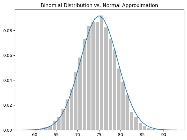
So to estimate the probability that a fair coin gives more than 60 heads in 100 flips, we can use $N(50, 5)$ instead of the binomial CDF. This is the basis of the tests in Hypothesis Testing.

Adapted from Joel Grus, Data Science from Scratch (2nd edition), chapter 6.

Original notebook

Tags: Statistics