GeoPandas and Projections

A GeoDataFrame is a pandas DataFrame with a special geometry column. Each entry is usually a Point, LineString or Polygon (or a Multi- version), and each type has attributes for quick analysis:

POI_data["geometry"].x         # x coordinate of each Point
roads_trails["geometry"].length  # length of each LineString
lands_data["geometry"].area      # area of each Polygon

These come back in the units of the coordinate reference system, which is why the next section matters.

Layers plot on the same axes like any matplotlib plot. Here are wild lands, campsites and foot trails in New York State, from the Kaggle geospatial course data:

fig, ax = plt.subplots(figsize=(8, 8))
counties.plot(color="none", edgecolor="grey", zorder=3, ax=ax)
wild_lands.plot(color="lightgreen", ax=ax)
campsites.plot(color="maroon", markersize=2, ax=ax)
trails.plot(color="black", ax=ax)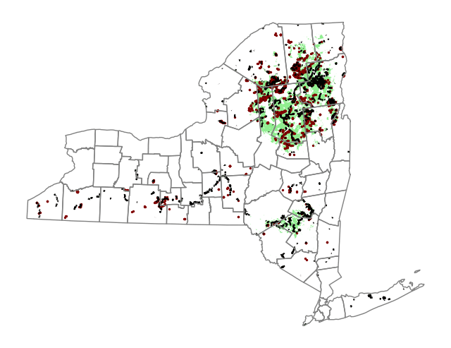

Coordinate reference systems

A map projection puts the curved surface of the Earth onto a flat one. None is perfect; each distorts something to preserve something else:

• Equal-area projections (Lambert Cylindrical Equal Area, Africa Albers Equal Area Conic) preserve area, so use them to measure the area of a country.
• Equidistant projections (Azimuthal Equidistant) preserve distance from a centre point, so are good for flight distances.
• Conformal projections (Mercator, Transverse Mercator) preserve local angles and shapes, so are good for navigation.

A coordinate reference system (CRS) says how the coordinates map to places on Earth. CRSs are usually identified by EPSG codes (from the European Petroleum Survey Group).

• EPSG:4326 is plain latitude and longitude on the WGS 84 datum. Units are degrees, so lengths and areas computed in it are meaningless.
• EPSG:32630 is WGS 84 / UTM zone 30N, a Transverse Mercator projection for 6° W to 0° (it covers Ghana and the UK). Units are metres. The original notes called this "the Mercator projection", which it is not: Transverse Mercator wraps the cylinder around a meridian, not the equator, so within its narrow zone distortion is tiny (a scale error of at most about 0.1%).

Reading a shapefile brings its CRS with it. Building a GeoDataFrame from a CSV of coordinates does not, so you have to set it:

facilities = gpd.GeoDataFrame(
    facilities_df,
    geometry=gpd.points_from_xy(facilities_df["Longitude"], facilities_df["Latitude"]),
    crs="EPSG:4326",
)

Note points_from_xy takes longitude first, because x is east–west.

Re-projecting

Layers must share a CRS before you plot or compare them. to_crs() changes only the geometry column:

regions.plot(color="none", linestyle=":", edgecolor="black", ax=ax)
facilities.to_crs(epsg=32630).plot(markersize=1, ax=ax)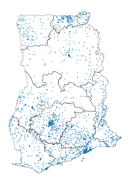

If there is no EPSG code for the CRS you want, to_crs() also takes a PROJ string, such as "+proj=longlat +ellps=WGS84 +datum=WGS84 +no_defs" for latitude and longitude.

Measuring area

Area in a projected CRS comes out in the CRS's units squared:

regions["area"] = regions["geometry"].area / 10**6  # square kilometres
regions["area"].sum()  # about 239,585

Ghana's official area is about 238,500 km², so UTM gives a close answer here. For areas across larger regions, re-project to an equal-area CRS first. The original notebook measured South America in EPSG:3035, which is the Lambert equal-area projection for Europe. Use one centred on the region instead, such as South America Albers Equal Area Conic:

south_america["geometry"].to_crs("ESRI:102033").area.sum() / 10**6

Lines from points

A sequence of points can become a path. With GPS tags from purple martins (11 birds, one reading roughly every two weeks):

paths = birds.groupby("tag-local-identifier")["geometry"].apply(lambda pts: LineString(list(pts)))
starts = birds.groupby("tag-local-identifier")["geometry"].first()
ends = birds.groupby("tag-local-identifier")["geometry"].last()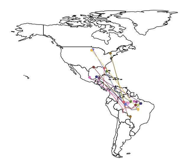

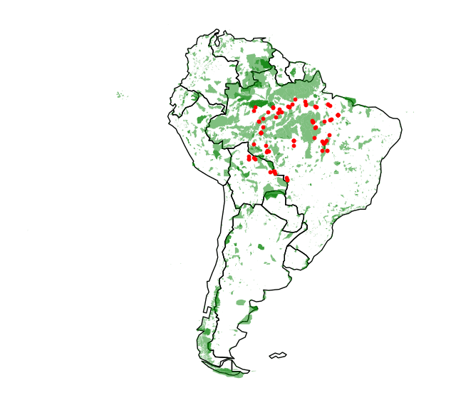
Overlaying the birds' southern-hemisphere readings on South America's protected areas shows where they spend the winter relative to protection:

Interactive maps with Folium

Folium draws Leaflet maps in a notebook. It wants coordinates in latitude and longitude (EPSG:4326).

m = folium.Map(location=[42.32, -71.0589], tiles="cartodbpositron", zoom_start=12)  # Boston

location is [latitude, longitude], here 42.32° N, 71.0589° W (the original said "-71.0589° E", which is the same point written confusingly). The main layers:

• folium.Marker: one pin per point. Wrap them in folium.plugins.MarkerCluster when there are many.
• folium.Circle: a bubble map; vary radius and color with other variables.
• folium.plugins.HeatMap(data=df[["Lat", "Long"]], radius=10): density. Larger radius is smoother.
• folium.Choropleth: colour areas by a value.

folium.Choropleth(
    geo_data=districts.__geo_interface__,  # GeoJSON, indexed by district
    data=crimes["DISTRICT"].value_counts(),  # Series with the same index
    key_on="feature.id",
    fill_color="YlGnBu",
    legend_name="Major criminal incidents (2018)",
).add_to(m)

key_on="feature.id" works because __geo_interface__ uses the GeoDataFrame's index as each feature's id, which is why the data Series must share that index. If you pass GeoJSON with the key in a property instead, use something like "feature.properties.DISTRICT".

Continues in joins and proximity.

Condensed from Kaggle's Geospatial Analysis course.

Original notebook · Folium notebook

Tags: Data Science, Geospatial