Image Processing

Contours with OpenCV

A contour is a curve joining the continuous boundary points of a region with the same colour or intensity. Contours are useful for shape analysis and object detection.

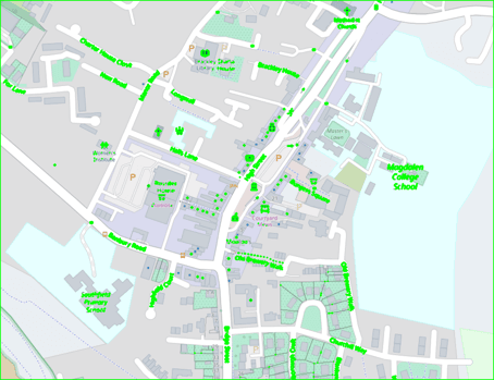
The usual recipe is: load, convert to greyscale, threshold to a binary image, find contours, draw them. The image is a map of Brackley (map data © OpenStreetMap contributors).

img = cv2.imread("brackley_map.png")  # note: OpenCV loads channels as BGR
grey = cv2.cvtColor(img, cv2.COLOR_BGR2GRAY)
_, thresh = cv2.threshold(grey, 127, 255, cv2.THRESH_BINARY)
contours, hierarchy = cv2.findContours(thresh, cv2.RETR_TREE, cv2.CHAIN_APPROX_SIMPLE)
cv2.drawContours(img, contours, -1, (0, 255, 0), 3)  # -1 draws them all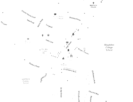

Thresholded at 127

All contours in green

Things to know:

• Use a binary image. Threshold or run Canny edge detection first.
• OpenCV finds white objects on a black background. On this map the background is light, so the threshold leaves a white background with dark text. The contours therefore trace the outer frame and the holes in it, i.e. the text, which happens to be what the plot shows. If you want the dark things as objects, invert with cv2.THRESH_BINARY_INV.
• Retrieval mode (RETR_TREE, RETR_LIST, RETR_EXTERNAL, ...) controls which contours are returned and whether the nesting hierarchy is kept.
• Approximation method: CHAIN_APPROX_NONE stores every boundary point; CHAIN_APPROX_SIMPLE keeps only end points of straight runs, so a rectangle needs 4 points instead of hundreds.
• drawContours draws in place, so successive calls pile up on the same image. Draw on img.copy() to compare.
• To draw one contour, pass it in a list: cv2.drawContours(img, [contours[4]], 0, (0, 255, 0), 3).
• To display an OpenCV image with PIL or matplotlib, convert BGR to RGB first (cv2.cvtColor(img, cv2.COLOR_BGR2RGB)), or reds and blues swap.

Contour features

M = cv2.moments(cnt)
cx, cy = M["m10"] / M["m00"], M["m01"] / M["m00"]  # centroid
area = cv2.contourArea(cnt)                         # same as M["m00"]
perimeter = cv2.arcLength(cnt, True)                # True: closed contour
approx = cv2.approxPolyDP(cnt, 0.1 * perimeter, True)  # Douglas–Peucker

Image moments are weighted sums over the region's pixels, from which you get the area $M_{00}$ and the centroid $C_x = M_{10}/M_{00}$, $C_y = M_{01}/M_{00}$.

Contour approximation replaces a shape with one with fewer vertices, using the Douglas–Peucker algorithm, with epsilon the maximum distance from the original. It is the tool for turning a rough four-sided blob into a square. Applied to a small text contour (area 18 pixels) with epsilon at 10% of the perimeter, as in the original notebook, it collapses to a two-point line, which shows the epsilon is far too coarse for that shape.

Geometric transforms with scikit-image

The example image is skimage.data.text(), a photo of handwriting on a page.

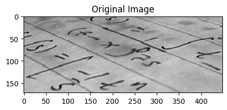
warp applies a transform to an image:

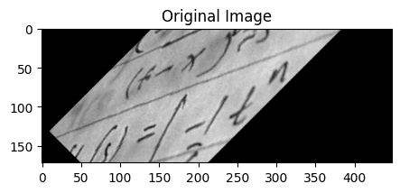
tform = SimilarityTransform(scale=1, rotation=math.pi / 4, translation=(img.shape[0] / 2, -100))
rotated = warp(img, tform)

That is a 45° rotation (π/4), not the 90° the original notes said.

Estimating a transform from control points

Usually you know where some points should end up rather than the transform's parameters. Given matching control points in two images, the parameters can be estimated by least squares. This is how image registration and rectification work.

Suppose we want to read text photographed at an angle. A flat page seen at an angle is a projective distortion, so a ProjectiveTransform can undo it. Mark the corners of a line of text (dst) and say where they should go (src): a 300 × 50 rectangle.

dst = np.array([[155, 15], [65, 40], [260, 130], [360, 95]])  # corners in the photo
src = np.array([[0, 0], [0, 50], [300, 50], [300, 0]])        # corners of the output
 
tform = ProjectiveTransform()
tform.estimate(src, dst)  # maps output coordinates -> input coordinates
warped = warp(img, tform, output_shape=(50, 300))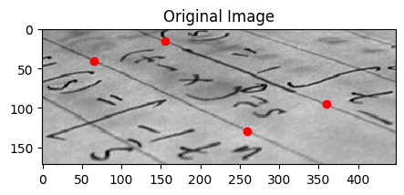

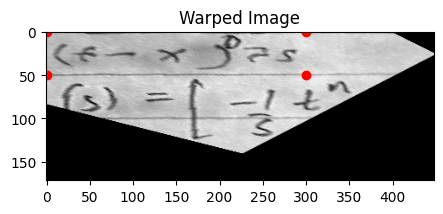
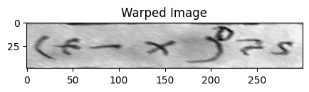
Control points on the photo

After warping

Why do the photo's points go in dst? It seems backwards, but warp works backwards on purpose: for each pixel of the output it asks which pixel of the input to sample. So the transform it needs maps output coordinates to input coordinates (its inverse_map), and estimating from src (output) to dst (input) gives exactly that. Working in that direction guarantees every output pixel gets a value, with no holes.

Partly condensed from the OpenCV contour tutorials and the scikit-image geometric transformation example.

OpenCV notebook · Image transforms notebook

Tags: Data Science, Computer Vision