Matplotlib

Figures and axes

fig, ax = plt.subplots()

The figure is the frame: you can resize it and save it, but you do not draw on it directly. An axes (a subplot) is one plotting area inside it, with its own x and y axis, title and data. A figure can hold many axes.

Matplotlib has two interfaces:

• pyplot (plt.plot, plt.xlabel, ...) acts on the "current" figure and axes, which matplotlib tracks for you. It is concise for a single quick plot.
• Object-oriented (ax.plot, ax.set_xlabel, ...) acts on the axes you name. It is clearer as soon as there is more than one plot, so it is the usual choice.

The original notes said pyplot "cannot create new axes or a new figure" and so fails when you add an unrelated plot. That is not right: plt.figure() and plt.subplot() create them, and plt.twinx() exists too. The TypeError in that example came from drawing dates onto an axes that already had a categorical (country name) x axis. The real argument for the object-oriented style is that you never have to wonder which axes is current.

Several subplots

fig, (ax1, ax2) = plt.subplots(1, 2, figsize=(10, 5))
ax1.plot(climate["date"], climate["co2"])
ax2.plot(climate["date"], climate["relative_temp"])
fig.tight_layout()

With more than one subplot, ax is a NumPy array of axes, so you can unpack it as above or index it (ax[0], or ax[0, 1] for a grid).

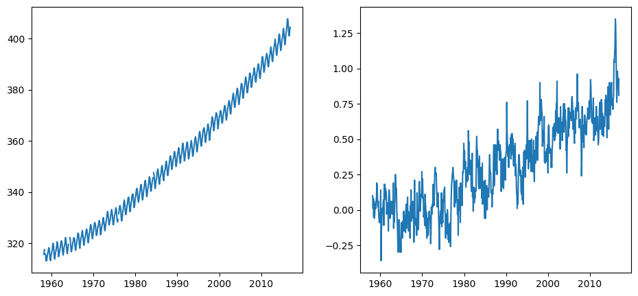
The data is monthly atmospheric CO₂ concentration (ppm, as measured at Mauna Loa) and relative temperature. The original called it CO₂ "emissions", but a concentration is not an emission.

ax.set(title=..., xlabel=..., ylabel=...) sets several properties at once. Use the individual ax.set_title(..., fontsize=20) methods when you need extra arguments. To rotate tick labels, prefer ax.tick_params(axis="x", labelrotation=90) over ax.set_xticklabels(..., rotation=90), which warns because it fixes the labels without fixing the tick positions.

Two y axes on one plot

ax.twinx() makes a second axes that shares the x axis but has its own y axis on the right (ax.twiny() is the reverse).

fig, ax = plt.subplots()
ax.plot(climate["date"], climate["co2"], color="blue")
ax2 = ax.twinx()
ax2.plot(climate["date"], climate["relative_temp"], color="red")
ax.tick_params("y", colors="blue")
ax2.tick_params("y", colors="red")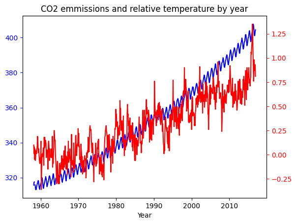

Twin axes are easy to misread, since the scales of the two y axes are arbitrary relative to each other. Colour-coding each axis to match its line helps.

Sharing axes between subplots

Comparing the 1980s with the 1990s side by side, each subplot picks its own y range, which hides the rise:

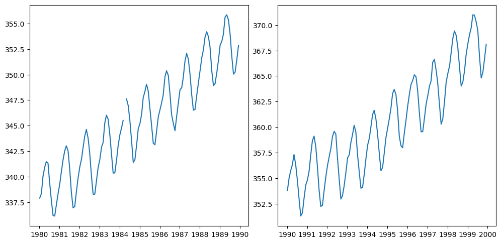
sharey=True puts them on the same scale:

fig, ax = plt.subplots(1, 2, figsize=(10, 5), sharey=True)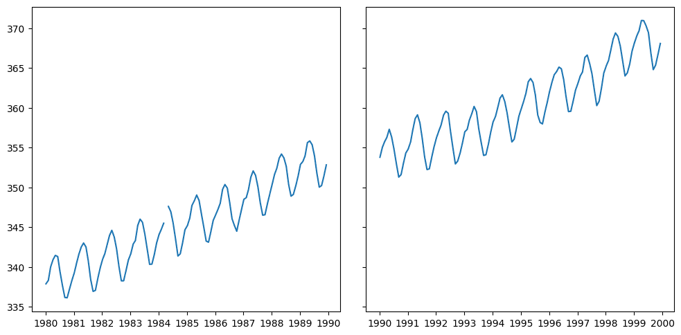

With time series, setting the date as the index (set_index("date"), or index_col in read_csv) makes slicing periods easy: climate["1980":"1989"].

Save a figure with fig.savefig("plot.png").

Adapted from a Towards Data Science article on matplotlib's figure and axes API.

Original notebook

Tags: Data Science, Visualisation