Microeconomics for Managers Chapter 2

2.1

(a)

Is row 1, column 2 a Nash equilibrium? (In all the strategic form games in these problems, the payoff of the person selecting the row is given first.)

No.

In game theory, a Nash equilibrium for a two-player game in normal form is a pair of strategies $(A,B)$ such that no player has incentive to unilaterally change her strategy. Formally, a strategy pair $(A, B)$ is a Nash equilibrium if:

$U_1(A, B) \geq U_1(A', B) \quad \text{for all } A' \text{ in the strategy set of player 1}$ $U_2(A, B) \geq U_2(A, B') \quad \text{for all } B' \text{ in the strategy set of player 2}$

Where $U_1$ and $U_2$ are the utility functions for player 1 and player 2, respectively. $A'$ and $B'$ refer to alternative strategies they could pursue.

For the row picking player, the best response to column 2 is row 2, not row 1.

(b)

Find all the Nash equilibria in the following game

In looking for Nash equilibria, we consider all possible strategies for both players, not just the ones that yield the highest payoffs in isolation. This is because a Nash equilibrium is defined as a situation where neither player has an incentive to unilaterally deviate from their current strategy, given the other player's strategy.

1. Row 1, Column 2 as a Nash Equilibrium:
   • If Row chooses row 1, the best response for Column is column 2 (payoff 2), and if Column chooses column 2, the best response for Row is row 1 (payoff 3). Neither has an incentive to deviate, so this is a Nash equilibrium.
2. Row 2, Column 1 as a Nash Equilibrium:
   • If Row chooses row 2, the best response for Column is column 1 (payoff 10), and if Column chooses column 1, the best response for Row is row 2 (payoff 5). Again, neither has an incentive to deviate, so this is a Nash equilibrium.
3. Row 3, Column 3 as a Nash Equilibrium:
   • If Row chooses row 3, the best response for Column is column 3 (payoff 5), and if Column chooses column 3, the best response for Row is row 3 (payoff 10). Neither has an incentive to deviate, so this is a Nash equilibrium.

2.2

Find all the Nash equilibria in the following game

Row 2 Column 2 and Row 4 Column 4. Following the same process as above...

1. If Row chooses row 1, Column will choose either column 1 or 2, either way Row will then choose row 2. Column will then chose column 2. So row 2, column 2 is a Nash equilibrium.
2. If Row chooses row 2, Column will choose column 2, row will then choose row 2. So we come to the same equilibrium as before.
3. If Row chooses row 3, Column will choose column 1, Row will then choose row 2, Column will then choose column 2. So we are again at the same equilibrium as before.
4. If Row chooses row 4, Column will choose column 3, Row will then stick with row 3. So this is also a Nash equilibrium.

2.3

Apply iterated dominance to the following game

Iterated dominance is a process used to simplify the strategic form of a game by iteratively eliminating dominated strategies. A strategy $A$ is said to be dominated if there is another strategy $A'$ that yields a higher payoff for all possible strategies chosen by the opponent.

If you find a strategy that is strictly dominated, you can remove it from the table. If this then results in another strategy becoming strictly denominated by another you can elimate that as well and so on.

Column 2 is dominated by column 4 because $1 < 3$, $1 < 2$, $0 < 1$ so can remove it:

Now row 3 is dominated by row 1 so we can remove it

Now column 1 is dominated by column 3 so we remove it

Now row 2 is dominated by row 2 so we remove it

Finally column 3 is dominated by column 4 and we are left with our equilibrium payoffs

When a game is dominance solvable using (at each step) strict (iterated) dominance, what remains is the unique Nash equilibrium of the game. More generally, any strategy eliminated by iterated strict dominance cannot be part of any Nash equilibrium.

2.4

Apply iterated dominance to the following game

In this game, there is no immediate strict dominance of any row or column.

Column 4 is weaky dominated by columns 1 and 2 and row 3 is weakly dominated by row 1. So we could remove column 4 and row 3

We probably shouldn't proceed any futher here. In game theory, a strategy is said to "weakly dominate" another if it is at least as good in all scenarios and better in at least one. Iterated dominance generally refers to the iterative elimination of strictly dominated strategies, not weakly dominated ones. While some forms of iterated dominance can include weak dominance, it's often avoided for a couple of reasons:

1. Ambiguity: Weakly dominated strategies can sometimes be part of a Nash equilibrium. Eliminating them might remove some Nash equilibria from consideration, thus making the analysis less robust.
2. Complexity: Including weak dominance can complicate the analysis and make it more difficult to find a clear, unequivocal solution.

In the real world the decision on whether or not to proceed would probably be decided by the emperical evidence available to you.

2.5

Imagine you are taking part in an auction, where the object being auctioned is a vacation trip. There are 15 other prospective buyers in addition to you. You have determined that the trip is worth $2000 to you: You would rather have the trip and pay some amount less than $2000 than to miss the trip (and pay nothing), but you would rather miss the trip (and pay nothing) than take the trip if it costs more than $2000. You are indifferent between missing the trip and paying nothing and going on the trip if it costs $2000.

To be very specific, your payoff is

• 0 if you do not win the auction (and pay nothing)
• $2000 - P$ if you win the trip and pay $P$.

You have very little idea how much the trip is worth to the other 15 bidders or how they bid.

(a)

Suppose this is a first-price auction. Why does the strategy of bidding $1950 weakly dominate the strategy of bidding $2000 for you? Can you compare (using dominance) bidding $1950 or bidding $1960? Can you compare (using dominance) bidding $2000 and bidding an amount more than $2000?

In a first-price auction, the highest bidder wins the item and pays the amount they bid.

Bidding $1950 vs. $2000:

• If you win at $1950, your payoff is $2000 - 1950 = 50$
• If you win at $2000, your payoff is $2000 - 2000 = 0$

Clearly, the payoff from winning at $1950 is better than or equal to winning at $2000 in every scenario, and it's strictly better in at least one scenario (when you win).

• If you lose at both $1950 and $2000, your payoff is 0 in either case.

Again, the payoff from bidding $1950 is at least as good as bidding $2000.

So, we can conclude that the strategy of bidding $1950 weakly dominates the strategy of bidding $2000.

Bidding $1950 vs. $1960:

• If you win at $1950, your payoff is $2000 - 1950 = 50$
• If you win at $1960, your payoff is $2000 - 1960 = 40$

Neither of these strictly dominates the other because the outcome depends on the bids of the other players. If the second-highest bid is between $1950 and $1960, then bidding $1960 would win you the auction while $1950 would not. However, you'd prefer to win at $1950 if possible due to the higher payoff. In this case, we can't say that one strategy dominates the other strictly or weakly; they are simply different strategies with different risks and rewards.

Bidding $2000 vs. Bidding more than $2000:

• If you win at $2000, your payoff is $2000 - 2000 = 0$.
• If you win at more than $2000 (say, $2050), your payoff would be negative (e.g. $2000 - 2050 = -50$).

Here, bidding $2000 strictly dominates bidding more than $2000 because in all scenarios, your payoff from bidding $2000 is at least as good as bidding more than $2000, and in some scenarios (when you win), it's strictly better.

(b)

Suppose this is a second-price (Vickery) auction. Why does the strategy of bidding $2000 weakly dominate every other strategy for you?

In a second-price auction, the highest bidder wins the item but pays the amount of the second-highest bid. Bidders have an incentive to bid their true valuation because they know they will only pay the second-highest price if they win, which will always be less than or equal to their own bid (and therefore less than or equal to their valuation).

Let's consider why bidding your true valuation of $2000 weakly dominates every other strategy for you:

1. If you bid less than $2000 (say, $1950) and win:
   • The second-highest bid must be less than or equal to $1950. You would have won even if you bid $2000, but by bidding less than your true valuation, you risk losing the auction to someone who might bid between $1950 and $2000, a range where you'd still consider the item worth buying.
2. If you bid $2000 and win:
   • You pay the second-highest price, which is less than or equal to $2000. This is your true valuation, so you are indifferent or happy with this outcome.
3. If you bid more than $2000 (say, $2050) and win:
   • You risk overpaying for the item. If the second-highest bid is between $2000 and $2050, you end up paying more than your valuation, which is undesirable.
4. If you lose the auction:
   • Your payoff is zero, regardless of what you bid, as long as the bid is less than or equal to $2000.

Therefore, by bidding your true valuation ($2000), you ensure that you win the auction whenever it's beneficial for you to do so (i.e., when the second-highest bid is less than $2000). You also avoid the risk of overpaying or underbidding. Hence, bidding $2000 weakly dominates all other strategies in a second-price auction for you.

2.6

Here are two extensive-form games of complete and perfect information: the threat game and the trust game. Solve each by backward induction. Then, do you think that your peers, playing the games in, say, units of $1 equals one unit of payoff, would follow the prediction of the Nash equilibrium analysis?

The threat game

If A is challenged, it will acquiesce. So B chooses between challenging and getting 1, and not challenging and getting 0. B will challenge A, and A will acquiesce.

The trust game

If B trusts A, A will act abusively (2 > 1). So B must choose between trust, getting -1 for itself, and no trust, which nets it 0. It will not trust A, and A will have no opportunity to move.

2.7

Imagine two firms, labeled $A$ and $B$, producing products that are substitutes but not perfect substitutes. The inverse demand functions for their two goods are $p_A = a - x_A - bx_B$ and $p_B = a - x_B - bx_A$ for a positive constant $a$ and for $0 < b < 1$, with the same constants $a$ and $b$ appearing in both inverse demand functions. Each firm has a constant marginal cost of production $c$.

(a)

Suppose the two firms must simultaneously and independently choose quantities to produce, each without knowing what the other has chosen. What are (or is) the Nash equilibria of this game?

In plain English, the inverse demand function $p_A = a - x_A - bx_B$ says that the price $p$ firm $A$ can sell it's good is determined by:

• The postive constant $a$. This represents the intercept of the inverse demand curve. It could be interpreted as the maximum price consumers are willing to pay when no units of either good are produced.
• The quantity of the good firm $A$ produces is given by the term $x_A$. This value is negative as the more of a good is produced, the lower will be its price.
• The quantity of the good firm $B$ produces is given by the term $x_B$.This value is negative for the same reason as $x_A$. It is mutliplied by the term $b$ which effectively weights the effect of $x_B$ by how similar the two goods are to each other. i.e. if the two goods are actually quite dissimilar, the effect of firm $B$ making more will be quite small.

We want to know to know the equilibrium values for $x_A$ and $x_B$.

Let's start by writing down a pair of equations to describe each firm's profit, the profit functions. Intially we could say that each firm's profit will be the price they sell their goods minus the cost of manufacturing them, all multiplied by the quantity that is manufactured:

Now as described in the question above, the prices of $A$ and $B$'s goods are given by their inverse demand functions. So we can subsitute them into the profit functions:

In order to maximise their profits, each firm will produce a quantity such that it would make make less profit if it made any more or any less. If we imagine plotting the profit functions for various quantities, the peaks of the curves will be where their derivatives are 0.

So we can find out what those quantities $x_A$ and $x_B$ will be by calculating the derivatives, setting them equal to 0, and solving for for their respective own quantity terms. These are known as reaction functions (and also as first-order conditions for profit maximisation) as they describe the the quantity a firm will produce to maximise its profit in response to the quantity produced by the other firm.

Finally to find the Nash equilibrium it we solve the reaction functions simultaneously. We'll substitute the reaction function for x_A into the reaction function for $x_B$ and solve for $x_B$.

We then can then subsitute our result for $x_B$ into the reaction function for $x_A$.

This implies that in the Nash equilibrium, both firms will produce the same quantity of output, which is given by the expression $\frac{a - c}{b + 2}$. This result is consistent with the symmetric nature of the Cournot competition model when the firms have identical cost structures and face the same demand conditions.

We can plot a visualisation of this result like so. Note that in this plot we are assuming that $a = 10$, $b = 0.5$, and $c = 2$.

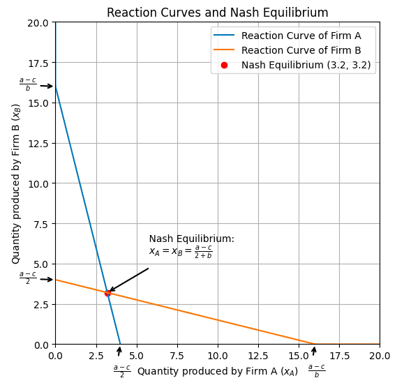
What is this showing us?

As the quantity produced by firm $B$ decreases, the optimal quantity for firm $A$ to make increases. If firm $B$ makes nothing at all the optimal quantity for firm A to make is:

Substituting our example values gives us $\frac{10 - 2}{2} = 4$ and indeed we can see that $x_A$ is 4 when $x_B$ is 0.

As the amount produced by firm $B$ increases, the optimal quantity form firm $A$ to produce decreases. At some point the optimal quantity for firm $A$ to make will be 0. Setting $x_A$ to 0 and rearranging to solve for $x_B$ shows us how much firm $B$ would have to make for this to be the case.

Substituting in our example values gives us $\frac{10 - 2}{0.5} = 16$ and indeed we can see that when $x_B$ is 16 $x_A$ is 0.

Of course, the same principles hold if with swap $A$ and $B$ around.

(b)

Suppose that the two firms must simultaneously and independently choose prices to charge, each without knowing what price the other has chosen. What are (or is) the Nash equilibria of this game?

First we find invert the inverse demand functions to get the demand functions.

We start by isolating the $x$ terms in each equation

We can then substitute the expression for $x_B$ into the expression for $x_A$

We can also say by symmetry that

We should also re-note the profit equations for each firm

Each firm will choose the price that maximises its profits given the price chosen by the other firm. We can substitute the demand functions that we have just derived into the profit functions

As in the last question we can find these "first order conditions for profit maximisation" by differentiating the profit functions with respect to the prices $P_A$ and $P_B$, and setting the derivatives equal to zero. First the derivative. To solve this we will need to make use of the quotient rule:

A this point I'm going to admit defeat regarding doing it by hand. Here's a way you can get the derivative using the Sympy library in Python

import sympy
 
pA, pB, a, b, c = sympy.symbols('pA pB a b c')
expression = (c*(a*(b - 1) - b*pB) + pA*(a*(1 - b) + b*pB + c) - pA**2)/(1 - b**2)
derivative = expression.diff(pA)
sympy.simplify(derivative)

What you'll get if you run this is the following expression:

And now, setting the derivate equal to zero

Because the firms respective functions are identical we can declare by symmetry that

As in the last question, to find the Nash equilibrium we have to solve these equations simulataneously. This time the algebra is even more of a nightmare to keep track of by hand so lets use a tool.

Wolfram Alpha has a tool for solving systems of equations here.

We can also use Sympy

import sympy as sp
 
pA, pB, a, b, c = sp.symbols('pA pB a b c')
 
eq1 = sp.Eq(pA, (a*(1 - b) + b*pB + c)/2)
eq2 = sp.Eq(pB, (a*(1 - b) + b*pA + c)/2)
 
solution = sp.solve((eq1, eq2), (pA, pB))

The solution from Sympy which can be multiplied by -1 to be the same as the solution in the textbook

We can visualise this. This plot shows pairs of prices each firm. Each line shows the best price of each firm to the corresponding price of the other firm. The place they intersect is the Nash equilibrium. Once again we assume that $a = 10$, $b = 0.5$, and $c = 2$.

Subsituting in 0 for $px_B$ allows us to predict what price firm $A$ would charge if firm $B$'s price was zero.

This is indeed where the line intersects the axis. The same is true when the firms are flipped.

(c)

Suppose Firm $A$ can choose its production quantity first. Firm $B$ sees this choice, then chooses its production quantity. What do you predict would happen?

This model is known as a Stackelberg competition. Once again the firms are trying to maximise their profits so we'll begin again by noting those profit functions and substituting in the inverse demand functions:

We first derived the reaction functions when looking at the Cournot competition model. We can do that again to see what firm $B$ will choose after seeing firm $A$'s production choice.

In a Stackelberg model though, firm $A$ anticipates this which means we need to update firm $A$'s profit function. We do this by substituting the reaction function into it.

This updated profit function is what we need to differentiate, set to 0, and rearrange to get the reaction function for firm $A$. Again, too much algebra for me to do by hand. However, we can use Sympy.

The expression for $x_A$ in the textbook is given as $\frac{\left(2 - b\right) \left(a - c\right)}{2(2 - 2 b^{2})}$. We can check that these are equivalent with Sympy:

book_answer = ((2 - b) * (a - c))/(2 * (2 - b**2))
reaction_a.equals(book_answer)

This evaluates to True.

We can substitute this into the reaction function for firm $B$ to find firm $B$'s equilibrium quantity.

Let's visualise this again.

We can plot the iso-profit curves for firm A alongside the reaction curves for the Cournot equilibrium. The iso-profit curve represents all the combinations of outputs (or other variables) that result in a specific level of profit $K$ that firm $A$ aims to achieve. Each point on an iso-profit curve corresponds to the same level of profit. The concept is similar to that of an isoquant in production theory, which represents all the combinations of inputs that result in a specific level of output.

Each iso-curve in this graph is described by the formula

We can read it as saying that that e.g. in a scenario where there firm $B$ is producing 8 units, firm A can make a profit of 4 by producing 2 units. Another way of putting this would be to say that if we substituted 2 substitued our constant values $a = 10$, $b = 0.5$, and $c = 2$ into the reaction function for firm $A$ and also substitute $x_B = 8$ we get

We can see from the left hand plot that the reaction curve for firm $A$ passes through the peak of firm $A$'s iso-curves.

The right hand plot shows the two reaction functions meeting at a point that in a Cournot model would result in a profit for A of ~10.24. In this scenario both firms have chosen their quantities simulataneously. The Nash equilibrium sees them both produce a quantity of 3.2. Under a Stackelberg model firm $A$ choses its quantity first. Firm $A$ knows that if it produces more than 3.2, firm $B$ will respond by producing less, something which benefits firm $A$.

We can find out how much more profit firm $A$ is able to make under this model by substiting our parameters into the equation for the equilibrium quanty for $x_A$ that we found above. This tells us how much firm $A$ will produce under this model

Substituting this value into the reaction function of firm $B$ tells us how much it will produce

Substituting $x_A$ and $x_B$ into the profit function for $A$ gives us

We can see that the iso-curve for $K = 10.29$ is the curve for which the reaction curve for firm $B$ is a tangent. Moving first has allowed firm $A$ to "move along" the curve to a more favourable pair of quantities. It has been able to increase its profit from 10.24 to 10.29.

(d)

Suppose Firm $A$ can choose its price first. Firm $B$ sees this choice, then chooses its price. What do you predict would happen?

TODO